Abstract
One of the greatest challenges in public health is the growing number of bacterial species that have developed resistance to antibiotics through point mutations in their genome. Our project aims to identify these genetic markers of antibiotic resistance through a genome wide association study between 36 antibiotic resistant E.Coli samples and 36 control samples. Genetic variants will be checked for statistical significance, and analyzed for any functional effects.
"By 2050, superbugs could kill 10 million people a year"
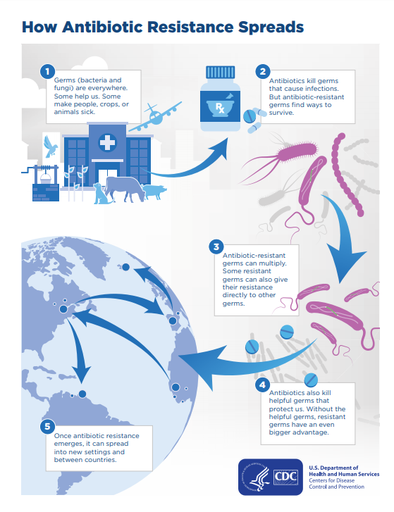
Although antibiotic resistant bacteria have been studied for decades, their whole genome sequencing has started relatively recently [3]. Due to their immunity to known medicine, their exposure to humans can lead to infections that are currently impossible to cure [1]. According to the International Federation of Pharmaceutical Manufacturers & Associations (IFPMA), antibiotic resistance will:
- Force 28 million more people into poverty[2]
- Cost the global economy up to 100 trillion dollars[2]
- Kill up to 10 million people a year by 2050[2]
This study focuses on Enterobacteriaceae, specifically E. Coli, a common cause of infections, both in healthcare settings and communities [4]. Certain strains of E. Coli have developed an especially dangerous resistance mechanism, the ability to produce an enzyme known as extended-spectrum beta-lactamase, or ESBL [4]. ESBL is capable of breaking down multiple types of antibiotics such as penicillin, rendering them ineffective [4].
Understanding the genetic markers of antibiotic resistance can lead to better, more effective treatments to combat the growing concern of superbugs.
Metholodgy
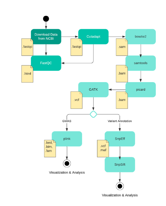
An Overview of the Pipeline
The Data
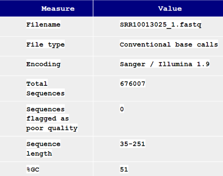
The study was conducted using two groups of samples, one with an ESBL-enzyme producing strain of E.Coli (denoted with DRR as the suffix), and a non-antibiotic resistant control group [5][6]. For each group, sample sizes were 36 whole genomes. The samples were obtained from NCBI's SRA Run Selector and formatted as .fastq files [5][6]. Each sample has two files associated with it, as they are paired-end reads, totalling to 144 files.
Quality Control
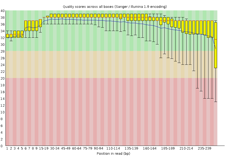
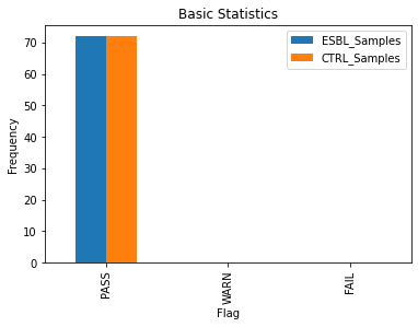
To ensure these 144 files will yield valid results later in the analysis, each was put through a quality control software called FastQC. FastQC takes in a single .fastq file and outputs a summary report listing basic statistics about the reads, including quality scores from base calling, the presence of adapter sequences, and percent N content which indicates missing data.
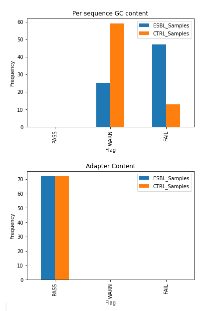
While it’s important to check for quality of each sample individually, the FastQC results of our case and control groups were also aggregated to identify any major differences in quality between the two that could affect the Genome-Wide Association Studies (GWAS) results. All 144 files passed the default FastQC check for basic statistics and adapter content, thus they were all included in the study. However, the antibiotic resistance group (ESBL) had more samples that had an unusually high per sequence GC content, indicated by the higher number of ESBL_Samples that failed this check (see GC and Adapter Content). This may either be a physiological phenomenon or a confounding factor that may need to be addressed.
During the sequencing process, temporary adapter sequences of nucleotides are attached to the fragments of DNA in order to facilitate sequencing [7]. Sometimes these adapters are accidentally sequenced as part of the sample genome, so they need to be algorithmically removed using tools such as Cutadapt. Cutadapt was run on all 72 samples using default parameters, in trimmed pair-end reads mode to “remove adapter sequences… from high-throughput sequencing reads”[8]. The trimmed fastq files were piped through FastQC again to ensure that the data still passes our quality check post-adapter trimming, which every file did [7].
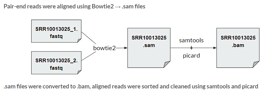
Sequence Alignment, File Conversion, Sorting
A pair of .fastq files for one sample contains the raw reads from the entire genome that need to be put together into a contiguous sequence. This is where the process of alignment comes in. Using a previously known E. Coli reference genome, we utilized an alignment software called Bowtie2 to algorithmically pieces together these reads. The outputs were 36 files in sam format, a text readable version of this sequence, per group (72 total). Using samtools and picard, these sam files were then converted to .bam files - a compressed version that runs more efficiently through bioinformatics software.
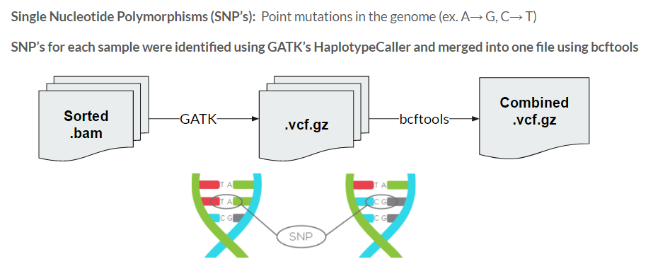
Variant Calling
The 72 cleaned and formatted .bam files then undergo variant calling, the process of identifying the Single Nucleotide Polymorphisms (SNP's) in each sample. These are the point mutations that can differentiate samples, with the goal being able to find the SNP’s that are significantly different between our antibiotic-resistant and control groups. This was done using GATK’s HaplotypeCaller tool, which outputs a vcf that contains the list of variants found in a single sample. All of these vcf files were then merged into a single file using bcftools to be applied for our GWAS.
Results
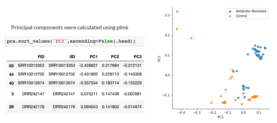
PCA Analysis
A basic Principal component analysis (PCA) was ran to determine if there were any meaningful difference between the Antibiotic-resistant and Control groups. The principle components were calculated using Plink and the initial results look promising, with most of the antibiotic-resistant E. Coli samples clustered together on the right. The control samples seem to have more variance, especially the three outliers in the top left. Due to our small dataset, the outliers were retained in the study.
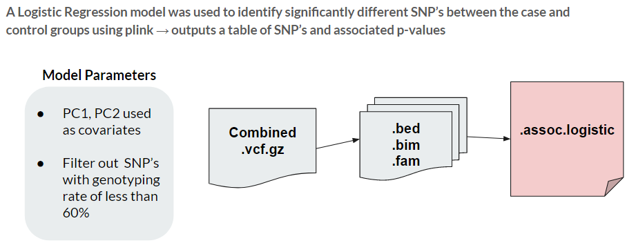
Genome Wide Association Study
In order to perform the GWAS, we used a Logistic Regression model, comparing the two groups and calculating a p-value for each SNP. The model was further tuned by utilizing the first two principal components as covariates, and removing all SNP’s with a genotyping rate of less than 60%. The genotyping rate is used as a measure of missing data, and we found that 60% was the best threshold to minimize the skew of our results.
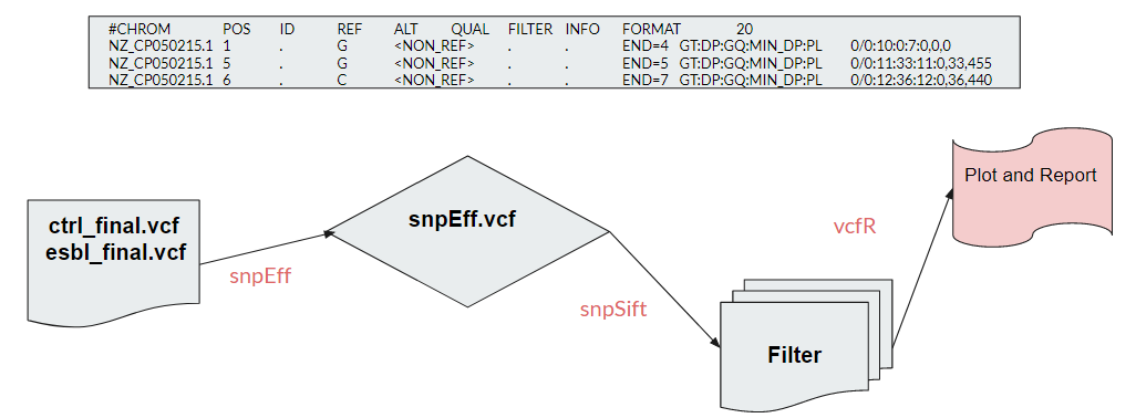
Variant Annotation
To perform further analysis on our variants, we chose snpEff to assist us with variant annotation. SnpEff provided us with an E. Coli database to use as the reference in our annotation, giving us an annotated vcf file, a succinct summary report, and gene_name table. We can then use snpSift to filter out the common variants present in both group, leaving only the necessary variants . This reduces the scope significantly and enables us to do more specific analyzation with it.
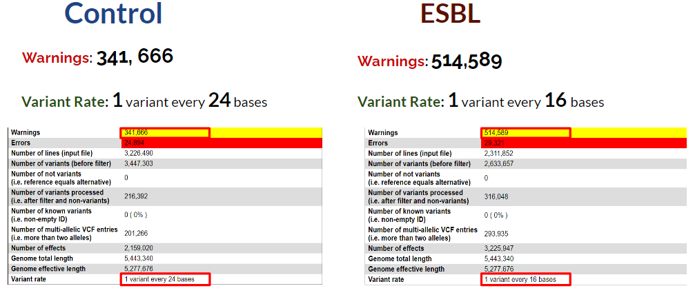
snpEff Summary
Since the number of errors we encountered is relatively small compared to our datasize, we decided to focus more on the numerous warnings. These warnings mainly consist of ref_dose_not_match_genome error. We theorized that it may be a result of using two different reference genomes: the original reference genome and the one provided by snpEff. It was unavoidable in this study as our initial reference genome was missing an essential .gff file. Our results could significantly improve if we built our own database. Another observation is that the variant rate of the esbl group is much higher than the control group. We hypothesize that it is due to the possibility that the ESBL group is more prone to mutations.
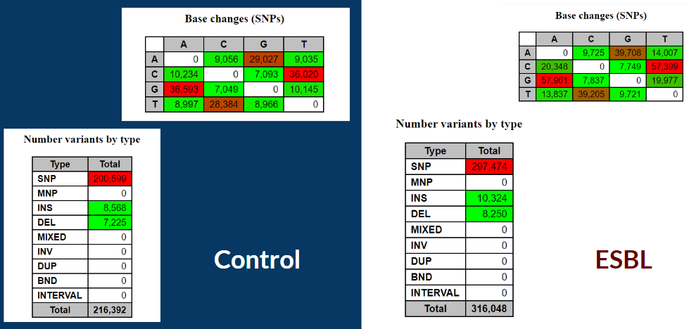
Overview of Variants
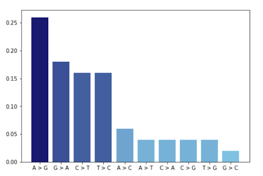
Below is brief overview of the base change and variants type of our two groups. Base change is a basic gene level mutation which alters the original gene base of a DNA molecule to another type (A --> C, etc). In the tables below, for both control and ESBL, one can observe that the most frequent base change happens between AG and CT and our variants consists of mainly SNP, with few insertion and deletion. In a study, G-C DNA was observed to "having a greater bonding between the base pairs" which implies that it is more difficult to have base changes between the pair and this can be clearly seen in our results[9].
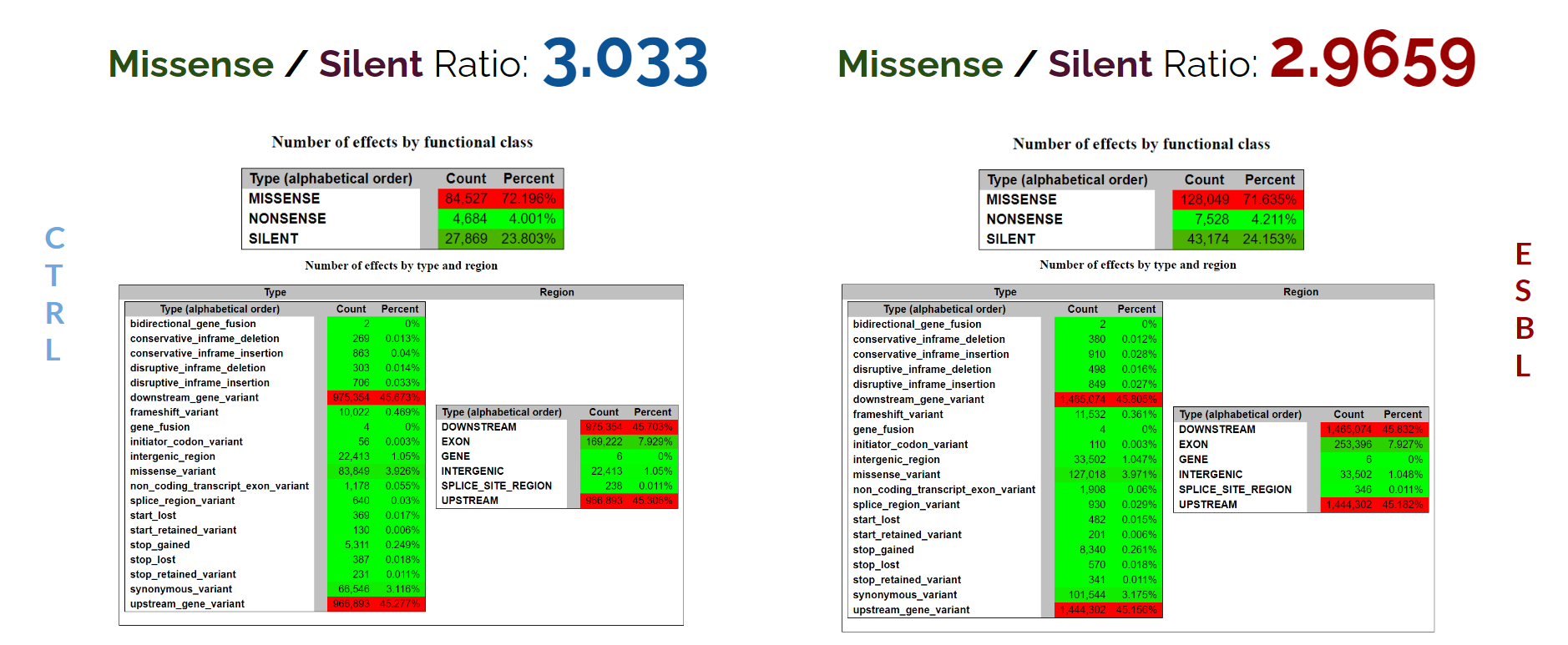
Possible Effects of Variants
The statistical data generated by snpEff illustrates that the control and ESBL group are incredibly similar with a few variance. For both groups, the Missense/Silent ratio is about 3 which is quite high. As this ratio increases, the more mutations happening in our samples directly affect the amino acid it produces. This could be reason for E. Coli bacteria gaining resistance to antibiotics. The rest of the statistics are similar and do not reveal how E. Coli bacterias become antibiotic resistant. Next, we will apply snpSift filtration to reduce the scope of the dataset to observe any noticeable changes.
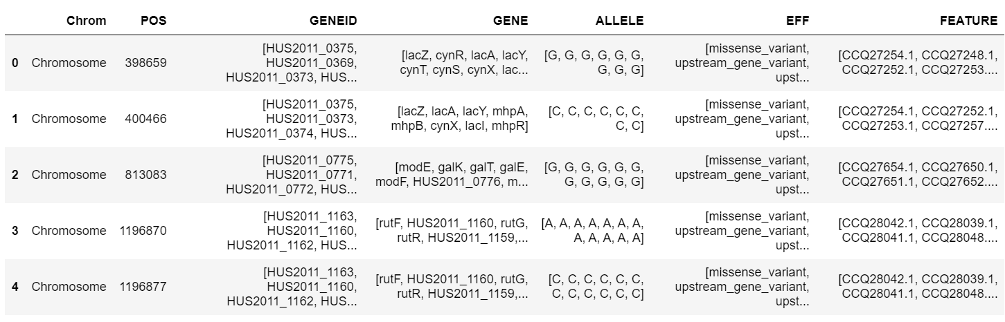
Finding the Mutated Genes
Using snpSift, only high/moderate impact variants (present in our ESBL samples and absent in at least one of our control samples) were kept. Originally, we had over 60 thousand variants, but only 50 remain after this filtration. Of those 50 variants, we extracted the top 10 most frequently found mutated genes. Below is a snippet of 5 variants that passed our filter.
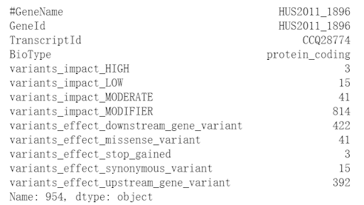
We can observe that in the remaining variants the most frequent mutations are from A -> G (see Base
changes). In addition, the variants_impact_MODIFIER is quite high indicating that there are more
variances,
with greater impact, in this gene.
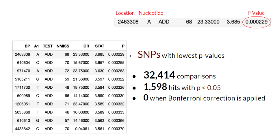
GWAS results
Here are the results of the GWAS Study done using logistic regression with Plink. The table is a list of SNP’s with the lowest p-values, indicating which variants are most likely to be statistically significant. 32,414 separate comparisons were made, with 1,598 variants having an associated p-value of less than 0.05. However, in studies dealing with biological data in particular, a technique called Bonferroni correction is applied due to multiple comparisons being done simultaneously. It’s calculated by dividing the desired threshold, 0.05, by the number of comparisons, resulting in a much smaller threshold. After applying this correction, 0 of these variants had p-values lower than this threshold.
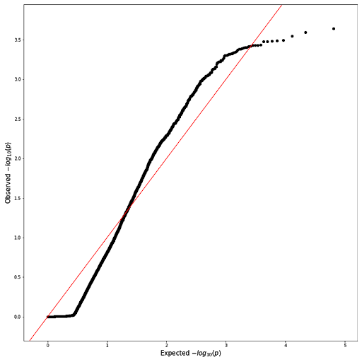
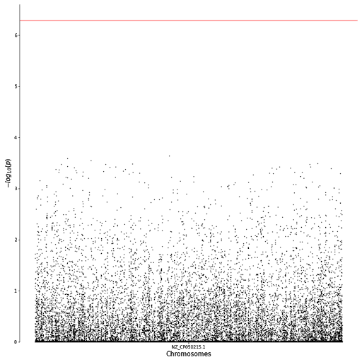
The p-values from the table were then visualized using a Q-Q plot to check if their distribution resembles data that is normally distributed. From the plot shown below (see Q-Q plot), there appears to be a skew of more extreme values, indicated by the longer tails at the ends. A Manhattan plot was also produced to visualize how these p-values vary across the genome. In the Manhattan plot, each dot represents a single SNP, with the -log10 of the p-value on the y-axis and the genome location on the x-axis. None of the SNPs hit the threshold for Bonferroni correction, indicated by the horizontal red line at the top of the plot (see Manhattan plot).
Conclusion
Our study aimed to explore and identify the genetic markers that characterize antibiotic resistance in ESBL-producing E. Coli. The project involved comprehensive processing of our genomic data, followed by a genome wide association study and analysis of found variants and their functional effects. Through our analysis, we noticed some observable differences through principal component analysis and variant annotation, but the location of the specific SNPs responsible for ESBL production is still unknown.
One of the primary limitations encountered was determining a definition for antibiotic resistance that could be feasibly tested using a GWAS. Although ESBL production has been proven to render E.Coli resistant to common antibiotics, there are many different physiological mechanisms that could also be used to classify other bacterial strains as antibiotic resistant. Another limitation was the limited sample size. This paired with the possible outliers from our principal component analysis could have given skewed results. If the study were to be repeated it would ideally involve hundreds, if not thousands of E.Coli samples. Time was another limiting factor, as a single sample takes approximately 60-70 minutes to be processed from raw reads to the Variant Call Format file needed for Plink and SnpEff. We also did not have access to a .gff file at the beginning of the study, which is an annotation file that is meant to be paired with the reference sequence used for alignment and variant calling. Because of this, we had to use two different reference genomes at different stages of the pipeline, which may have influenced the final GWAS and SnpEff outputs. In order to improve the logistic regression model, covariates such as %GC Content and more granular SNP filtering could be implemented.
This study is a small stepping stone toward addressing the much broader problem of antibiotic resistance. The project pipeline can be applied to any strain of bacteria with a case and control group which can not only help identify significant genomic variants, but also their effects on protein transcription. Understanding these markers for antibiotic resistance can better inform scientists of how such physiological changes occur and what can be done to prevent the emergence of new antibiotic resistant strains in the future. Testing resistance to specific drugs can drive the development of new and effective treatments by pharmaceutical companies. A machine learning model can apply our pipeline to more easily identify and predict whether a new bacterial strain has the potential to be antibiotic resistant.
Sources
-
Citations
1. Center for Disease Control. “About Antibiotic Resistance.” Centers for Disease Control and Prevention, Centers for Disease Control and Prevention, 13 Mar. 2020, www.cdc.gov/drugresistance/about.html#:~:text=Antibiotic%20resistance%20happens%20when%20germs,and%20sometimes%20impossible%2C%20to%20treat.
2. Cueni, Thomas B. “By 2050, Superbugs May Cost the Economy $100 Trillion.” IFPMA, International Federation of Pharmaceutical Manufacturers & Associations , 13 Nov. 2018, www.ifpma.org/global-health-matters/by-2050-superbugs-may-cost-the-economy-100-trillion/#:~:text=Antimicrobial%20resistance%20(AMR)%20is%20on,%E2%80%9Csuperbugs%E2%80%9D.
3. Ikegawa, Shiro. “A short history of the genome-wide association study: where we were and where we are going.” Genomics & informatics vol. 10,4 (2012): 220-5. doi:10.5808/GI.2012.10.4.220
4. Center for Disease Control. “ESBL-Producing Enterobacteriaceae.” Centers for Disease Control and Prevention, Centers for Disease Control and Prevention, 22 Nov. 2019, www.cdc.gov/hai/organisms/ESBL.html.
5. Patel, IR. National Center for Biotechnology Information, U.S. National Library of Medicine, 22 May 2015, trace.ncbi.nlm.nih.gov/Traces/study/?acc=PRJNA230969&o=acc_s%3Aa.
6. Hokkaido University. National Center for Biotechnology Information, U.S. National Library of Medicine, 8 Dec. 2020, trace.ncbi.nlm.nih.gov/Traces/study/?acc=PRJDB10450&o=acc_s%3Aa.
7. Babraham Institute. Babraham Bioinformatics - FastQC A Quality Control Tool for High Throughput Sequence Data, 26 Apr. 2010, www.bioinformatics.babraham.ac.uk/projects/fastqc/.
8. Cutadapt — Cutadapt 3.1 documentation.https://cutadapt.readthedocs.io/en/stable/
9. "DNA Structure - The School Of Biomedical Sciences Wiki". Teaching.Ncl.Ac.Uk, 2021, https://teaching.ncl.ac.uk/bms/wiki/index.php/DNA_Structure?fbclid=IwAR00bHpJnec5eIT31PAJPRufMWzlob86-cJiY-rfdRGFC7Py3AT1ueOcZ3w.
- Source Code